Financial Review using Natural Language Processing

What is Natural Language Processing (NLP) ?

Natural Language Processing (NLP) is a branch of artificial intelligence that helps computers understand, interpret, and generate human language—just like we do when we speak, write, or read.

How does it work?

Together, these allow machines to:

• Break down sentences into parts (syntax)

• Understand meaning and context (semantics)

• Respond or generate text that feels natural

About the dataset: I took the financial dataset from the market and performed the index rate , and reviewed the comments using NLP

Step 1: Import the required libraries

import numpy as np
import pandas as pd
import matplotlib.pyplot as plt
import seaborn as sns


plt.style.use('ggplot')
import nltk

Step 2: Read the dataset

financial_data = pd.read_csv('/Users/FinancialNews/financial_news_events.csv')

financial_data.head()

Remove the NaN values using dropna() and ensure all the values are properly removed

financial_new_df = financial_data.dropna()

financial_new_df.isna().sum()
Date                    0
Headline                0
Source                  0
Market_Event            0
Market_Index            0
Index_Change_Percent    0
Trading_Volume          0
Sentiment               0
Sector                  0
Impact_Level            0
Related_Company         0
News_Url                0
dtype: int64

financial_new_df.head()

financial_new_df.shape
(2443, 12)

financial_new_df.ndim
2

Step 3: Perform the quick EDA

financial_new_df['Index_Change_Percent'].value_counts().sort_index().plot(kind = 'bar',title = ' Count of Trading Volume by Population',
                                                                    figsize= (10,5))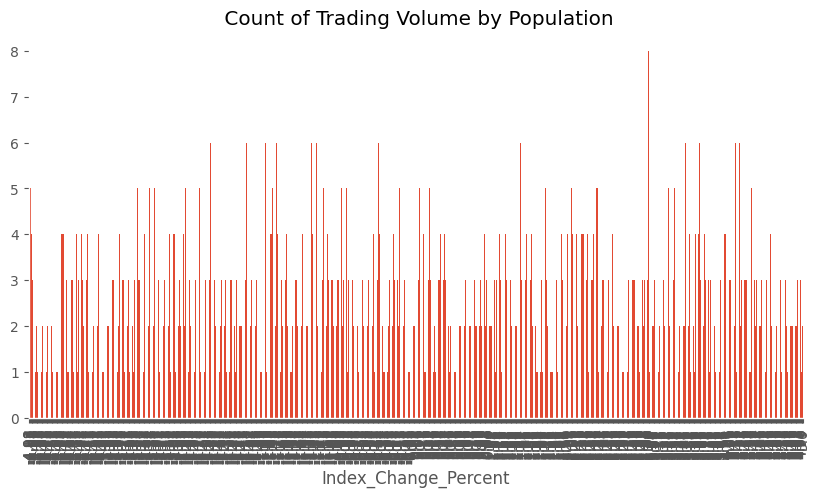

Step 4 : Basic NLTK using example object and taken sample sentences from the main dataset

from nltk.tokenize import word_tokenize

example = financial_new_df['Headline'][500]
print(example)

tokens = nltk.word_tokenize(example)

print(tokens)
['Consumer', 'confidence', 'index', 'reaches', 'a', 'decade', 'high']

tokens[:3]
['Consumer', 'confidence', 'index']

tagged = nltk.pos_tag(tokens)

tagged[:10]
[('Consumer', 'NNP'),
 ('confidence', 'NN'),
 ('index', 'NN'),
 ('reaches', 'VBZ'),
 ('a', 'DT'),
 ('decade', 'NN'),
 ('high', 'JJ')]

entities = nltk.chunk.ne_chunk(tagged)

entities.pprint()
(S
  (GSP Consumer/NNP)
  confidence/NN
  index/NN
  reaches/VBZ
  a/DT
  decade/NN
  high/JJ)

Step 5: Sentimental Analysis: VADER sentiment scoring method

from nltk.sentiment import SentimentIntensityAnalyzer

from tqdm.notebook import tqdm

sia = SentimentIntensityAnalyzer

Note: Polarity Scores define negative, neutral and positive measures. Compound score between -1 to +1

sia().polarity_scores(example)
{'neg': 0.0, 'neu': 0.471, 'pos': 0.529, 'compound': 0.5423}

financial_new_df.head()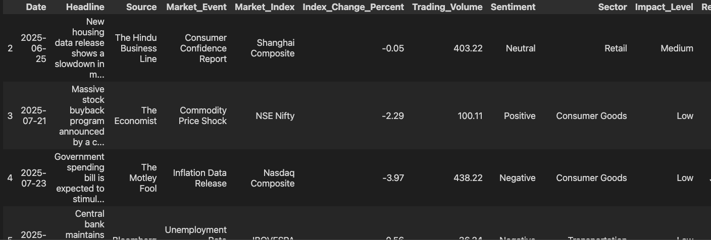

Step 6 : Run the polarity score on the entire dataset

### Run the polarity score on the entire dataset
res = {}
for i, row in tqdm(financial_new_df.iterrows(), total = len(financial_new_df)):
    text = row['Headline']
    myid = row['Index_Change_Percent']
    res[myid] = sia().polarity_scores(text)
    break

res = {}
for i, row in tqdm(financial_new_df.iterrows(), total=len(financial_new_df)):
    text = row['Headline']
    myid = row['Index_Change_Percent']
    res[myid] = sia().polarity_scores(text)

res

{-0.05: {'neg': 0.0, 'neu': 1.0, 'pos': 0.0, 'compound': 0.0},
 -2.29: {'neg': 0.0, 'neu': 0.659, 'pos': 0.341, 'compound': 0.4767},
 -3.97: {'neg': 0.0, 'neu': 1.0, 'pos': 0.0, 'compound': 0.0},
 0.56: {'neg': 0.0, 'neu': 0.745, 'pos': 0.255, 'compound': 0.34},
 -3.68: {'neg': 0.0, 'neu': 1.0, 'pos': 0.0, 'compound': 0.0},
 -4.33: {'neg': 0.0, 'neu': 1.0, 'pos': 0.0, 'compound': 0.0},
 3.35: {'neg': 0.0, 'neu': 1.0, 'pos': 0.0, 'compound': 0.0},
 -1.66: {'neg': 0.0, 'neu': 0.769, 'pos': 0.231, 'compound': 0.4588},
 -2.45: {'neg': 0.0, 'neu': 1.0, 'pos': 0.0, 'compound': 0.0},
 0.92: {'neg': 0.0, 'neu': 1.0, 'pos': 0.0, 'compound': 0.0},
 2.83: {'neg': 0.0, 'neu': 1.0, 'pos': 0.0, 'compound': 0.0},
 -2.92: {'neg': 0.0, 'neu': 1.0, 'pos': 0.0, 'compound': 0.0},
 4.41: {'neg': 0.0, 'neu': 1.0, 'pos': 0.0, 'compound': 0.0},
 4.15: {'neg': 0.0, 'neu': 1.0, 'pos': 0.0, 'compound': 0.0},
 -0.95: {'neg': 0.0, 'neu': 0.732, 'pos': 0.268, 'compound': 0.296},
 -2.37: {'neg': 0.0, 'neu': 1.0, 'pos': 0.0, 'compound': 0.0},
 -1.96: {'neg': 0.0, 'neu': 1.0, 'pos': 0.0, 'compound': 0.0},
 4.28: {'neg': 0.0, 'neu': 1.0, 'pos': 0.0, 'compound': 0.0},
 -2.02: {'neg': 0.0, 'neu': 0.714, 'pos': 0.286, 'compound': 0.4215},
 1.34: {'neg': 0.0, 'neu': 1.0, 'pos': 0.0, 'compound': 0.0},
 -1.18: {'neg': 0.0, 'neu': 1.0, 'pos': 0.0, 'compound': 0.0},
 2.46: {'neg': 0.0, 'neu': 1.0, 'pos': 0.0, 'compound': 0.0},
 -4.4: {'neg': 0.0, 'neu': 0.745, 'pos': 0.255, 'compound': 0.34},
 3.53: {'neg': 0.0, 'neu': 0.741, 'pos': 0.259, 'compound': 0.2732},
 -3.44: {'neg': 0.0, 'neu': 0.714, 'pos': 0.286, 'compound': 0.4215},
...
 -4.92: {'neg': 0.0, 'neu': 0.66, 'pos': 0.34, 'compound': 0.5574},
 -1.97: {'neg': 0.0, 'neu': 0.745, 'pos': 0.255, 'compound': 0.34},
 4.25: {'neg': 0.0, 'neu': 1.0, 'pos': 0.0, 'compound': 0.0},
 1.79: {'neg': 0.216, 'neu': 0.784, 'pos': 0.0, 'compound': -0.296},
 -4.5: {'neg': 0.0, 'neu': 0.769, 'pos': 0.231, 'compound': 0.4588}}

Step 8: Make the res object into a Dataframe, so that it would be easy to merge with mthe ain dataset

vaders = pd.DataFrame(res).T
vaders.reset_index().rename(columns= {'index':'Id'})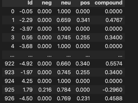

financial_new_df = financial_new_df.reset_index().rename(columns={'index': 'Id'})

Step 9: Now we have a sentimental score of metadata

vaders = vaders.merge(financial_new_df, how='left', left_index=True, right_on='Index_Change_Percent')

vaders.head()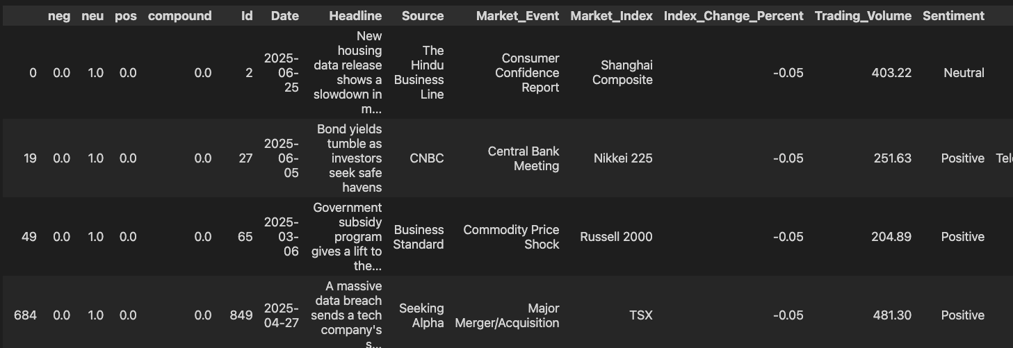

Step 10: Create Barplot and this plot gives the compound score. Compound score gives the entire persption of the sentence, if it is +1 which means positive and -1 means negative (customer not satisfied)

ax = sns.barplot(data = vaders, x = 'Index_Change_Percent', y = 'compound')
ax.set_title('Compound score by Financial dataset')
plt.show()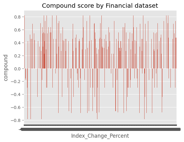

fig, axs = plt.subplots(1,3, figsize = (12,3))
sns.barplot(data=vaders,x = 'Index_Change_Percent', y = 'pos',ax = axs[0])
sns.barplot(data=vaders, x = 'Index_Change_Percent', y = 'neu', ax = axs[1])
sns.barplot(data=vaders, x = 'Index_Change_Percent', y = 'neg',ax = axs[2])
axs[0].set_title('Positive')
axs[0].set_title('Neutral')
axs[0].set_title('Negative')
plt.tight_layout()
plt.show()