Netflix Stock Price using Simple Linear Regression Model

About the dataset :

Linear regression is a supervised learning method that models the relationship between a dependent variable (such as Netflix’s closing stock price) and one or more independent variables (like opening price, high, low, volume, etc.). The goal is to find the best-fitting line that minimizes prediction error.

Target Variable: Closing price of Netflix stock (NFLX)

Features Used: Date, Open, High, Low, Close, Adjusted Close, Volume

Model Type: Simple or multiple linear regression depending on the number of predictors

Step 2 : Reading the Netflix object in detail

netflix.describe(include='all')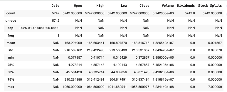

Step 3: Exploratory Data Analysis

netflix.isnull().sum()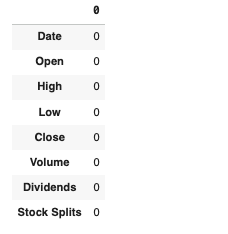

netflix.shape
(5742, 8)

netflix.size
45936

netflix.columns
Index(['Date', 'Open', 'High', 'Low', 'Close', 'Volume', 'Dividends',
       'Stock Splits'],
      dtype='object')

netflix.head()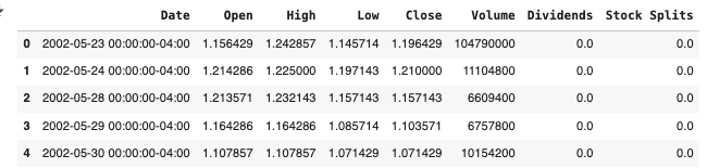

sns.pairplot(netflix)
plt.show()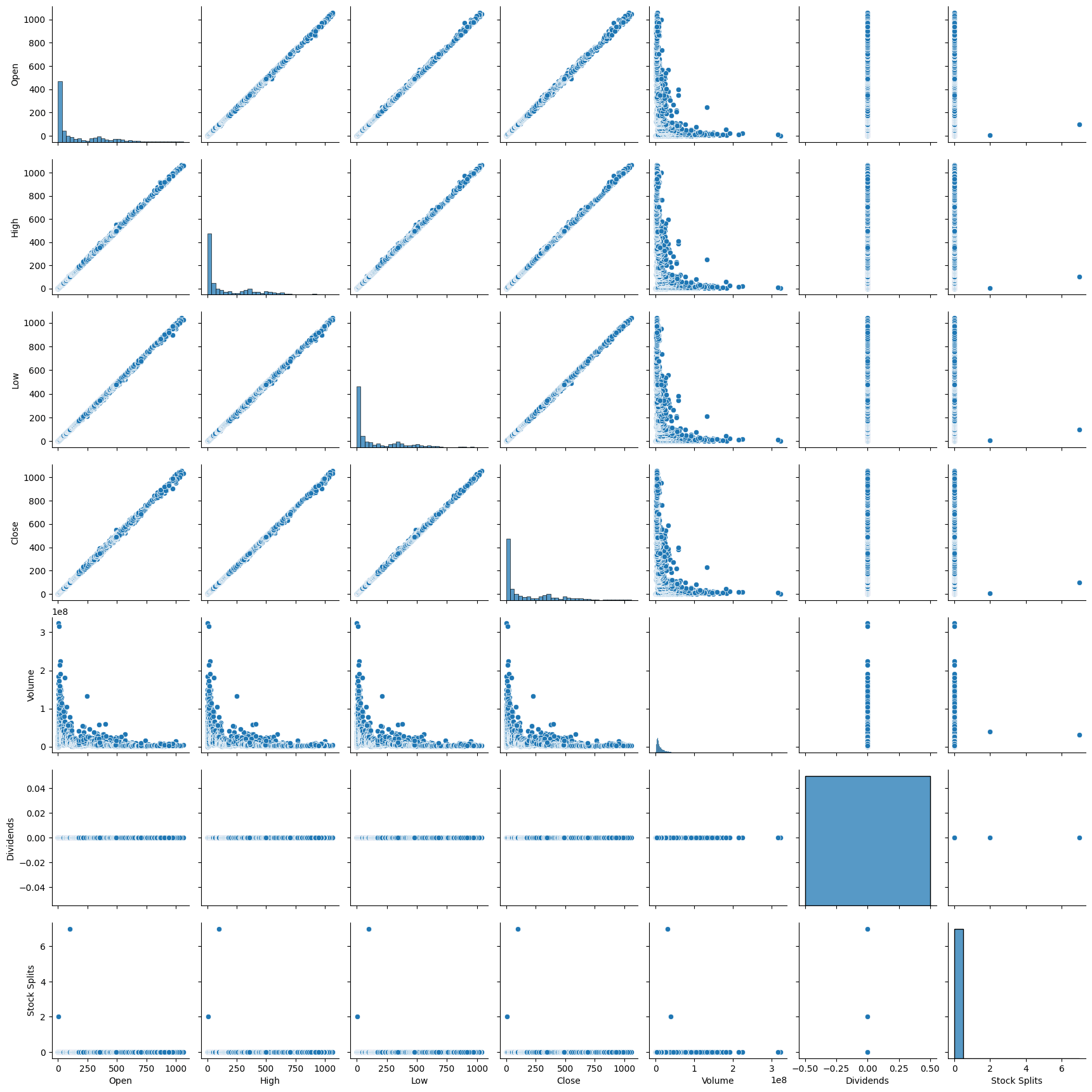

Step 4: Feature Selection from the main dataset - netflix

X = netflix[['Open', 'High', 'Low','Volume']].values
y = netflix['Close'].values

Step 5: Create a Linear Regression model using the above features

from sklearn.linear_model import LinearRegression

model = LinearRegression()
model.fit(X, y)
y_pred = model.predict(X)
residuals = y - y_pred

sns.histplot(residuals, kde=True)
plt.xlabel('Residuals')
plt.ylabel('Frequency')
plt.title('Histogram of Residuals')
plt.show()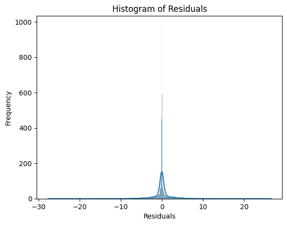

Step 5: Splitting the test and train data

from sklearn.model_selection import train_test_split

# split train and test data
x_train, x_test, y_train, y_test = train_test_split(X, y, test_size=0.2, random_state=42)

from sklearn.linear_model import LinearRegression

lm = LinearRegression()
lm.fit(x_train, y_train)

lm.coef_

Step 6: Score the linear model

#values from 0 to 1
#0 model explain None of the variability
#1 model explain Entire of the variability
lm.score(x_train, y_train)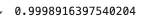

predictions = lm.predict(x_test)

from sklearn.metrics import mean_squared_error,mean_absolute_error,r2_score

r2score = r2_score(y_test, predictions)
r2score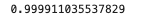

dframe=pd.DataFrame({'actual':y_test.flatten(),'Predicted':predictions.flatten()}) 

dframe.head(15)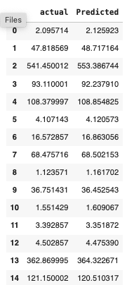

Step 7: Plot the graph

# Plotting the graph
sns.pairplot(dframe)
plt.show()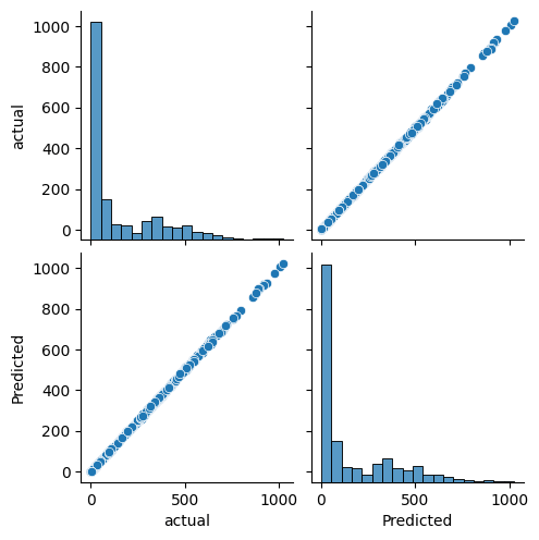

graph = dframe.head(15)
graph.plot(kind='bar',figsize=(10,8))
plt.title("Actual vs Predicted")
plt.xlabel("Actual Data")
plt.ylabel("Closing Price")
plt.show()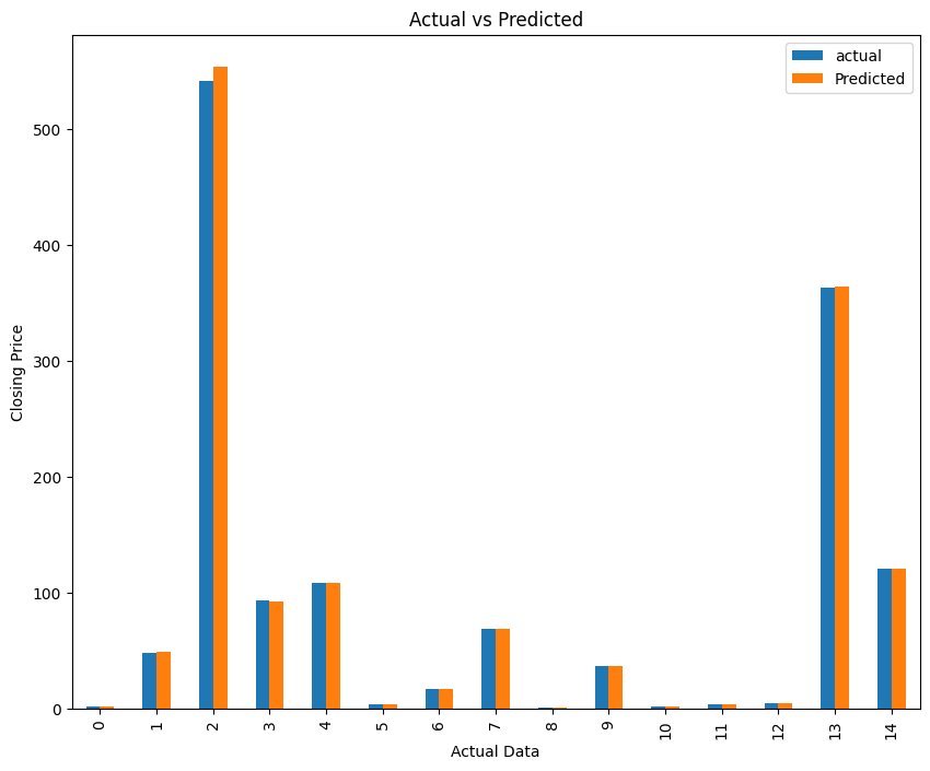

fig = plt.figure()
plt.scatter(y_test, predictions)
fig.suptitle('Actual vs Predicted', fontsize=20)               # Plot heading 
plt.xlabel('Actual', fontsize=18)                               # X-label
plt.ylabel('Predicted', fontsize=16)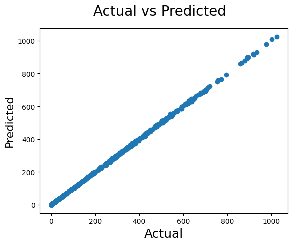

sns.regplot(x=y_test,y=predictions,ci=None,color ='red')
plt.xlabel('Actual')
plt.ylabel('Predicted')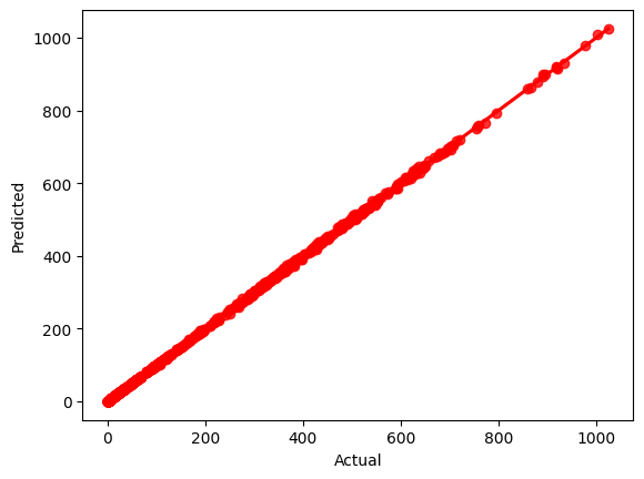

import math 
from sklearn import metrics

print ("Mean absolute error ", mean_absolute_error(y_test, predictions))
print ("Mean squared error ", mean_squared_error(y_test, predictions))
print ("Root mean squared error ", math.sqrt(mean_squared_error(y_test, predictions)))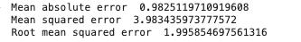

Conclusion :

MAE 0.98 On average, your model's predictions are off by about 0.98 units from the actual values. This is a direct, intuitive measure of error. MSE 3.98 The average of the squared errors. This penalizes larger errors more heavily, suggesting that some predictions may be significantly off. RMSE 1.99 The square root of MSE, bringing the error back to the original unit. It indicates that, on average, predictions deviate from actual values by about 1.99 units.