About the dataset :

This dataset is designed for beginners in Machine Learning who want to practice building classification models. It contains 1,000 anonymized patient records, each with medical and demographic features commonly associated with diabetes diagnosis.

Apply explanation techniques to an already trained model. These methods treat the model as a black box but seek to explain its behaviour after the fact. Post-hoc techniques can be model-agnostic (applicable to any model type) or model-specific. They include methods like:

• Feature importance**: Evaluate which features most affect the model’s predictions. For instance, permutation importance measures how the model’s error changes when a feature’s values are randomly shuffled.

Partial dependence plots (PDPs): Show the relationship between a particular feature and the predicted outcome, averaging out the effects of other features. This gives a global view of how changing that feature influences predictions.

Local explanation methods**: Explain individual predictions.

• LIME (Local Interpretable Model-agnostic Explanations) approximates the model locally with a simple surrogate model to explain why a specific prediction was made.

  • SHAP*(Shapley Additive exPlanations) assigns each feature a contribution value for a given prediction, based on cooperative game theory, offering consistency in how feature impacts are computed. These methods help answer “why did the model predict X for this instance?” by attributing portions of the prediction to features.

Method 1: Post Hoc - Partial Dependency Plot

Step 1 : Importing Required Libraries and packages

Step 2 : Reading the dataset using Pandas:

Step 3: Exploratory Data Analysis using the same dataset

diabetes_data.head()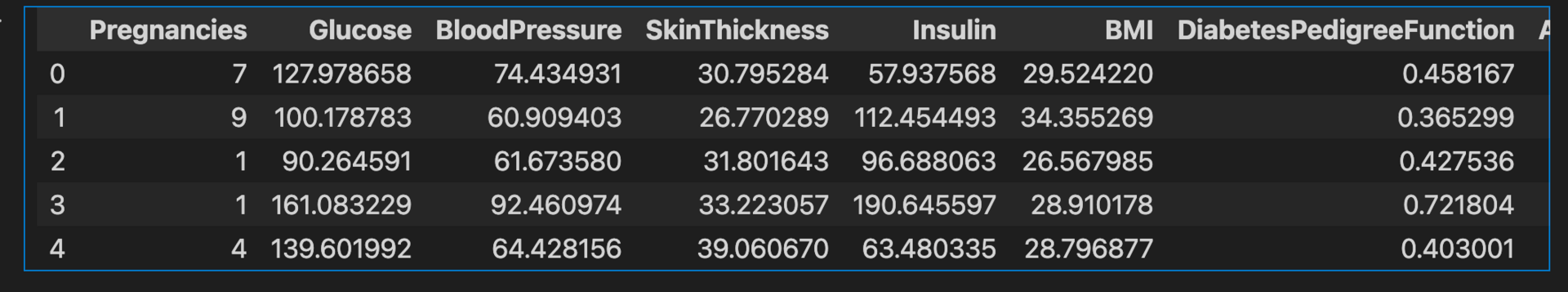

diabetes_data.describe()

diabetes_data.info()

diabetes_data.isna().sum()

diabetes_data.value_counts

diabetes_data.shape
(964, 9)

Step 4: Split the X and Y, segregate the required features for each variable

X = diabetes_data.drop('Outcome', axis=1)
y = diabetes_data['Outcome']

Step 5: Train a simple model

model = RandomForestRegressor(random_state=42)
model.fit(X, y)

Step 6: Create a features object and define it from the main dataset

featues = diabetes_data[["BMI","Glucose"]]

Step 7: Create Partial Dependence Plot

#Partial Dependence Plot for BMI:
PartialDependenceDisplay.from_estimator(model,X, featues, 
                                        kind="average",
                                        grid_resolution=50)
plt.title("Partial Dependence Plot for BMI")
plt.show()

Method 2: Post HOC - Permutation Feature Importance

import pandas as pd
import numpy as np
import matplotlib.pyplot as plt
from sklearn.ensemble import RandomForestRegressor
from sklearn.ensemble import RandomForestClassifier
from sklearn.model_selection import train_test_split
from sklearn.inspection import permutation_importance
from sklearn.metrics import mean_squared_error, r2_score,accuracy_score

X = diabetes_data.drop('Outcome', axis=1)
y = diabetes_data['Outcome']

### Train / Test Split: 
X_train, X_test, y_train, y_test = train_test_split(X, y, test_size=0.2, random_state=42)

### Fit a Random Forest Model 
model = RandomForestClassifier(random_state=42)
model.fit(X_train, y_train)

### Baseline Accuracy:
print("Baseline Accuracy:", accuracy_score(y_test, model.predict(X_test)))
Baseline Accuracy: 0.48704663212435234

### Permutation Importance 
importance_diabetes = permutation_importance(model, X_test, y_test, n_repeats=10, random_state=42)

print(importance_diabetes)
'importances_mean': array([ 0.01398964, -0.00362694, -0.03626943,  0.02746114, -0.02435233,
        0.02124352, -0.00777202, -0.03626943]), 'importances_std': array([0.01911489, 0.01410431, 0.01622018, 0.02329302, 0.01671737,
       0.02191532, 0.01969594, 0.02419195]), 'importances': array([[ 0.02072539,  0.02072539,  0.00518135,  0.00518135,  0.05181347,
        -0.01036269, -0.01554404,  0.02590674,  0.00518135,  0.03108808],
       [-0.01554404, -0.01554404,  0.00518135,  0.00518135, -0.01554404,
         0.        ,  0.01554404,  0.02072539, -0.02072539, -0.01554404],
       [-0.02072539, -0.01036269, -0.05699482, -0.06217617, -0.02590674,
        -0.03108808, -0.03108808, -0.04663212, -0.02590674, -0.05181347],
       [ 0.        ,  0.06735751,  0.02072539,  0.03626943, -0.01554404,
         0.02590674,  0.04663212,  0.05181347,  0.01554404,  0.02590674],
       [-0.01554404, -0.05699482, -0.03626943, -0.00518135, -0.02590674,
        -0.00518135, -0.01554404, -0.02590674, -0.04663212, -0.01036269],
       [ 0.00518135, -0.02590674,  0.03108808,  0.03108808,  0.04663212,
         0.01554404,  0.01554404,  0.03626943,  0.05181347,  0.00518135],
       [-0.00518135, -0.03626943, -0.02072539,  0.01036269, -0.02072539,
         0.02072539,  0.01554404,  0.01036269, -0.03108808, -0.02072539],
       [-0.06217617, -0.05699482, -0.07253886, -0.02072539, -0.05699482,
        -0.02072539, -0.01036269, -0.01554404,  0.        , -0.04663212]])}

plt.figure(figsize=(10,6))
plt.barh(X.columns, importance_diabetes.importances_mean)
plt.xlabel("Mean Decrease in Accuracy")
plt.title("Permutation Feature Importance for Diabetes Classification")
plt.show()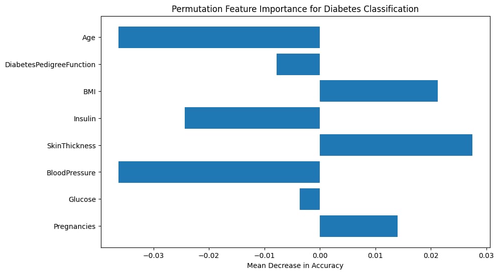

Method 3: Shapley Additive exPlanations

import pandas as pd
import shap 
import numpy as np
from sklearn.ensemble import RandomForestRegressor
from sklearn.inspection import permutation_importance
from sklearn.model_selection import train_test_split

X = diabetes_data.drop('Outcome', axis=1)
y = diabetes_data['Outcome']

model = RandomForestClassifier(random_state=42)
model.fit(X, y)

explainer = shap.TreeExplainer(model)
shap_values = explainer.shap_values(X)

shap.summary_plot(shap_values, X, plot_type="bar")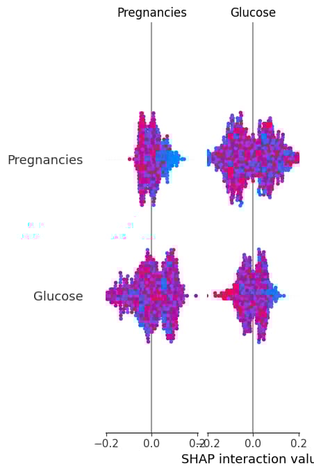

shap.initjs()
shap.summary_plot(shap_values, X)