Regression Model - Decision Tree using historical silver price

About the dataset :

A silver price dataset generally contains historical prices of silver, usually quoted in USD per troy ounce, and spans multiple years or even decades. These datasets help analysts study long‑term trends, volatility patterns, and relationships with macroeconomic factors.

Step 1: Importing Required Libraries and packages

Step 2: Reading the dataset using Pandas:

Step 3 : Perform the Exploratory Data Analysis

# Display the first few rows of the dataset
print(silver_data.head())

silver_data.info()

silver_data.isna().sum()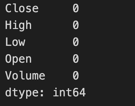

silver_data.describe()

Step 4: Split X and Y values to train and test the dataset

X = silver_data.drop('Open', axis=1)
y = silver_data['Open']

X.columns
Index(['Close', 'High', 'Low', 'Volume'], dtype='object')

Step 5: Perform the Standard Scaler step for normalization of the dataset

from sklearn.preprocessing import StandardScaler
scaler = StandardScaler()
X_scaled = scaler.fit_transform(X)
X_scaled[:3]

array([[-1.37281023, -1.36928184, -1.37862523,  0.10239238],
       [-1.36506253, -1.359309  , -1.37594111,  0.0186463 ],
       [-1.36495635, -1.36035879, -1.36896241, -0.00942699]])

Step 6: Now Split the train and test data with 80/20 or 70/30

from sklearn.model_selection import train_test_split
X_train, X_test, y_train, y_test = train_test_split(X_scaled, y, test_size=0.2, random_state=42)

X_train.shape 
(5078, 4)

y_train.shape
(5078,)

X_test.shape
(1270, 4)

y_test.shape
(1270,)

Step 6: Import the Decision Tree Regressor

from sklearn.tree import DecisionTreeRegressor
dt_regressor = DecisionTreeRegressor(random_state=42)
dt_regressor.fit(X_train, y_train)

y_predict = dt_regressor.predict(X_test)

Step 7: Import the required libraries to check the mean absolute error for both test and train datasets

from sklearn.metrics import mean_absolute_error, mean_squared_error, r2_score
mae = mean_absolute_error(y_test, y_predict)
mse = mean_squared_error(y_test, y_predict)
r2 = r2_score(y_test, y_predict)

mean_absolute_error(y_test, y_predict)
0.11038426301610747

y_predicted_train = dt_regressor.predict(X_train)
mae_train = mean_absolute_error(y_train, y_predicted_train)
mae_train
0.0

Step 8: Compare the Predicted Train and Predicted value and determine whether this is overfitting or underfitting.

y_predicted_train
array([ 8.81999969,  4.6420002 , 15.84500027, ..., 25.84000015,
       24.55500031,  6.579     ])

y_train
1328     8.820000
57       4.642000
3593    15.845000
3319    19.930000
6305    51.259998
          ...    
3772    14.510000
5191    27.285000
5226    25.840000
5390    24.555000
860      6.579000
Name: Open, Length: 5078, dtype: float64

Note: Based on the above comparison, it clearly shows it is “Overfitting” which means predicted_train and predicted value are exactly matching.

Step 9: Import the required libraries of GridSearchCV through sklearn

from sklearn.model_selection import GridSearchCV
param_grid = {
    'max_depth': [3, 5, 10],
    'min_samples_split': [2, 5, 10],
    'min_samples_leaf': [1, 2, 4]
}

rg1 = DecisionTreeRegressor()
rg1 = GridSearchCV(rg1,param_grid)

rg1.fit(X_train, y_train)

rg1.best_params_
{'max_depth': 10, 'min_samples_leaf': 2, 'min_samples_split': 2}

y_predict = rg1.predict(X_test)
mean_absolute_error(y_test, y_predict)
0.11820789700440988

y_predicted_train = rg1.predict(X_train)
mean_absolute_error(y_train, y_predicted_train)
0.055056556970567896

Conclusion: Using the GridSearchCV module helped correct the imbalance in the dataset and improved the model’s ability to generalize. After tuning the hyperparameters, the mean absolute error changed significantly, indicating that the model is now learning meaningful patterns rather than simply memorizing values from the predicted_train dataset.